This post may contain affiliate links
Table of Contents
🎧 Audio Discussion Available
An AI-generated podcast explores this article’s concepts through conversational debate format—useful for audio learners or those wanting to hear multiple perspectives.
Duration: 16 minutes
Crypto trading with hedge funds returns averaged 40%+ annual returns while you struggled to break even. They’re trading the same markets. The same Bitcoin. The same Ethereum. The same 24/7 chaos.
So what’s the difference?
Most assume it’s insider information, better connections, or secret strategies unavailable to retail traders. That’s comforting because it means the game is rigged and there’s nothing you could have done differently.
The uncomfortable truth: It’s systematic mathematics most traders never learn. The performance gap isn’t what they know—it’s what they systematize.
This article will show you the exact math that separates consistent winners from frustrated losers. No insider knowledge required. No million-dollar minimum investment. Just mathematics that have worked across every asset class, in every market, for over a century.
By the end, you’ll understand why professional crypto trading systems like HyperTrend achieve hedge-fund-level performance—and how the same mathematics can work for you.
The Performance Mystery: Why Returns Don’t Tell the Whole Story
Here’s a question most crypto traders get wrong:
Which investment is better?
- Investment A: 40% annual returns with 40% annualized volatility
- Investment B: 20% annual returns with 10% annualized volatility
Most people instantly choose A. Double the returns? Obviously better, right?
Wrong. Investment B is dramatically superior, and understanding why reveals the fundamental difference between amateur and professional thinking.
The Leverage-Invariant Secret
Professional traders don’t measure performance by returns alone—they measure returns per unit of risk. This is called the Sharpe ratio, and it’s the single most important concept separating retail from institutional approaches.
The Sharpe ratio formula (simplified): Returns ÷ Volatility
- Investment A: 40% ÷ 40% = 1.0 Sharpe ratio
- Investment B: 20% ÷ 10% = 2.0 Sharpe ratio
Why B is better: With Investment B’s superior risk-adjusted returns, you can apply 2x leverage to match Investment A’s absolute returns (20% × 2 = 40%) while maintaining lower volatility than A (10% × 2 = 20% vs. A’s 40%).
The result: Same returns, half the volatility, dramatically better long-term compounding.
This is what professionals mean by “leverage-invariant” performance measurement. A Sharpe ratio lets you compare strategies fairly regardless of how much leverage is applied.
Formula: (Return – Risk-Free Rate) / Volatility
Where:
- Return = Your annual percentage gain (e.g., 40%)
- Risk-Free Rate = Treasury bills (~4%) – baseline return without risk
- Volatility = Standard deviation of returns (how much it bounces around)
Example: Investment earning 40% with 40% volatility
(40% – 4%) / 40% = 0.9 Sharpe Ratio
Why it matters: Sharpe ratio above 1.0 = top 5% of hedge funds globally. HyperTrend targets 1.5+, placing it in institutional elite territory.
The Sharpe Ratio Hierarchy: Where Do You Stand?
Here’s how different strategies and investors stack up historically:
Sub-1.0 Sharpe (Underperforming):
- Treasury Bonds: 0.36
- Buy & Hold Stocks: 0.4
- Bitcoin (10-year hold): 0.81
1.0 Sharpe (Professional Grade):
- Ray Dalio: ~1.0
- George Soros: ~1.0
- Traditional volatility-targeted trend following: 1.0-1.2
1.5+ Sharpe (Institutional Elite):
- Finrev historical performance: 1.81
- Conservative forward estimate: 1.5
- Renaissance Technologies (after massive fees): 2.5
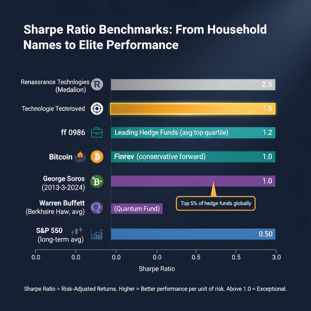
The benchmark that matters: A Sharpe ratio above 1.0 means you’re in the top 5% of hedge funds globally. A Sharpe ratio of 1.5+ puts you in elite institutional territory.
For context: Warren Buffett’s lifetime Sharpe ratio is 0.76. Bitcoin’s 10-year Sharpe ratio is just 0.81 despite life-changing absolute returns.
The math reveals an uncomfortable truth: even Bitcoin, despite making millionaires, delivered returns inefficiently. For every dollar of return, you endured more than a dollar of volatility.
Historical Sharpe ratios by investor/strategy:
- Warren Buffett (lifetime): 0.76
- Bitcoin (10-year hold): 0.81
- Ray Dalio / George Soros: ~1.0
- Traditional trend following: 1.0-1.2
- Finrev historical: 1.81
- Renaissance Technologies (after fees): 2.5
Context: A Sharpe ratio of 1.0 beats 95% of all hedge funds. Anything above 1.5 is exceptionally rare – typically only achieved by elite quant firms like Renaissance or D.E. Shaw. Sources: A Trend Following Deep Dive” (2026), Man Group Insights And: A Trend Following Deep Dive” (2026), Man Group Insights.
Why A Trend Following Crypto Strategy Amplifies the Advantage
Traditional markets can achieve Sharpe ratios of 1.0-1.2 with volatility-targeted trend following. In crypto, those same strategies can hit 1.5-1.8.
Why the difference?
- Higher base volatility: More price movement = more trends to capture
- Behavioural inefficiency: Immature market with more emotional trading
- 24/7 operation: Momentum compounds without daily reset interruptions
- Friction advantages: Moving money on/off exchanges creates sticky capital
- Lower institutional competition: Fewer sophisticated players hunting the same edges
The practical meaning: Take a trading strategy that delivers 30% annually with 25% volatility in traditional markets (1.2 Sharpe). Apply it to crypto. Expect 40-50% annually with 30% volatility (1.5+ Sharpe).
Link to HyperTrend evolution: This is why rebuilding on Hyperliquid infrastructure matters. Same Sharpe expectations, but 15-20% better execution efficiency = compounding advantages that separate winners from almosts.
The Timeline Problem: Why Patience Isn’t Optional
Here’s the part that destroys most traders: even with a 1.5 Sharpe ratio system, short-term results look nearly random.
Professional trading firms run Monte Carlo simulations—generating thousands of possible outcome paths based on historical statistics—to understand performance timelines. The results are sobering.
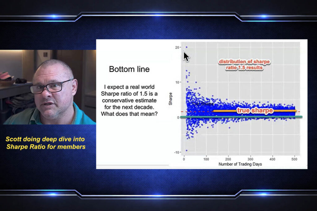
What to Expect After 50 Trading Days (2-3 Months)
With a 1.5 Sharpe ratio system (better than 95% of hedge funds), after 50 trading days:
- Top 10% outcome: Excellent profits, everything working perfectly
- Average outcome: Slightly positive, but noisy and unconvincing
- Bottom 10% outcome: Losses
One-third of the time, you’ll be losing money after 50 days with a world-class system. This is normal statistical variance, not system failure.
Look at any trading forum. Someone launches a system, shows 50 days of great results, and everyone piles in. Three months later, it’s underperforming, and everyone exits. They captured the lucky top 10% outcome window and mistook it for skill.
What to Expect After 100 Trading Days (4-5 Months)
The picture improves but remains frustrating:
- Results spread widely around the expected average
- Still possible (though less likely) to be in a drawdown
- Not yet clear if you’re experiencing bad luck or a broken system
The psychological trap: This is when most traders quit. They see others’ “better” systems (probably just luckier timing) and jump ship right before their system works.
What to Expect After 200 Trading Days (8-10 Months)
Finally, clarity begins to emerge:
- Strong convergence toward the expected Sharpe ratio
- Obvious separation between working systems and broken ones
- Still some outcomes significantly above/below average (luck still matters)
What to Expect After 300 Trading Days (12-15 Months)
This is the minimum timeline for judgment:
- Results cluster tightly around the true Sharpe ratio
- Very unlikely to be losing money with a 1.5 Sharpe system
- Luck becomes noise rather than a dominant factor
- You can confidently assess if the system works
The brutal reality: You need a minimum of 12-15 months to judge a trading system’s true performance. Anything shorter, you’re mostly measuring luck.
Why this matters: When HyperTrend launches with its improved execution infrastructure, don’t expect instant results. The mathematics don’t change. What changes is long-term compounding efficiency as better execution compounds over these 12-15 month (and longer) timelines.
With a world-class 1.5 Sharpe system (better than 95% of hedge funds), after 50 trading days:
- 33% chance you’re LOSING money
- 33% chance you’re slightly positive
- 33% chance you’re doing great
One-third of the time, excellence looks like failure in the short term.
Why retail traders fail: They see 50 days of losses, assume the system is broken, and quit right before it works. They see someone else’s lucky 50-day run and chase it right before regression to mean.
The fix: Minimum 12-15 months (300+ trading days) to judge ANY trading system’s true performance. Anything shorter is measuring luck, not skill. Source: The Evaluation and Optimization of Trading Strategies (2nd Edition) by Robert Pardo
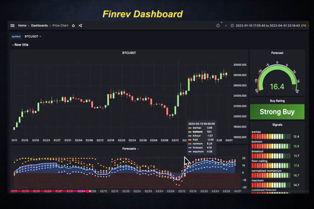
The Six Signals: How Professional Systems Actually Work
Most retail bots rely on 1-3 indicators. Professional systems blend dozens of uncorrelated signals. Here’s what Finrev (the foundation of HyperTrend) actually trades:
Signal #1: Exponentially Weighted Moving Average (EWMA) Crossovers
- What it is: Fast-moving average crosses above/below slow moving average
- Timeframes used: 2/8, 4/16, 8/32, 16/64, 32/128, 64/256 day pairs
- Origin: Man AHL (one of the world’s largest trend-following hedge funds)
- Why it matters: 80% of professional CTA (Commodity Trading Advisor) trend following hedge funds use this as their primary signal. It’s not secret sauce—it’s the industry workhorse because it works consistently across all markets.
The key innovation: Rather than binary “long when fast > slow,” the system calculates signal strength from the distance between moving averages. Wider separation = stronger signal = larger position.
Signal #2: Bollinger Band Momentum
- What it is: Measures the distance between the current price and the 2-standard deviation Bollinger bands
- Why it works: Extreme deviations from “normal” price ranges predict continuation
- The edge: Most traders use Bollinger bands for mean reversion (“price is stretched, it’ll snap back”). Professional systems recognize that extreme stretches in trending markets predict continuation, not reversion.
Signal #3: Breakout Systems
- What it is: New 10, 20, 40, 80, 160, or 320-day highs/lows
- Why it works: Breakouts to new highs attract momentum buyers; breakdowns create panic selling
- Cost structure: Shorter breakouts (10-day) trigger more trades = higher costs. Longer breakouts (320-day) trade rarely but capture major trends. The system blends all timeframes with cost-adjusted weights.
Signal #4: Laurent Bernut Floor-Ceiling (Regime Detection)
- What it is: Proprietary regime detection from Laurent Bernut’s Fidelity hedge fund days
- Why it matters: Detects when markets shift from trending to ranging behaviour
- The advantage: Most systems trade the same way in all conditions. This signal adjusts when market structure changes.
Signal #5: Normalized Momentum (Rob Carver Methodology)
- What it is: Smoothed momentum calculation before generating trading signals
- Origin: Rob Carver, ex-Man AHL trader
- The innovation: Traditional momentum is noisy. Smoothing first, then calculating momentum, reduces false signals without sacrificing predictive power.
Signal #6: MACD Momentum (Man AHL Variation)
- What it is: Modified MACD (Moving Average Convergence Divergence) approach
- Origin: Published by an ex-Man AHL trader in a research paper
- Why it’s different: Not the MACD retail traders know from TradingView. This institutional variation focuses on longer-term convergence/divergence patterns.
Why 6 Signals Instead of 1?
Diversification of strategy timeframes.
- Fast signals (2/8 EWMA, 10-day breakout) catch early momentum
- Slow signals (64/256 EWMA, 320-day breakout) ride sustained trends
- Regime detection (floor-ceiling) adjusts when behavior shifts
The mathematics of signal blending: Two uncorrelated signals performing at 1.2 Sharpe each will create a combined system with ~1.5 Sharpe. Three signals push to ~1.6 Sharpe. By six signals, you’re approaching 1.8 Sharpe.
Diminishing returns: Adding signal 7, 8, 9 helps less and less. But those first 6 do the heavy lifting.
Link to HyperTrend expansion: With semi-HFT execution, previously untradeable signals (too fast, too expensive) become viable. HyperTrend plans 50-100+ signals by expanding into shorter timeframes that infrastructure couldn’t support before.
Kelly Criterion: The Math of Optimal Position Sizing
The question every trader faces: How much should I risk on each trade?
The wrong answers:
- “Risk 2% per trade” (arbitrary, ignores strategy quality)
- “Risk whatever feels right” (emotional, inconsistent)
- “Risk everything” (ruin guaranteed)
The right answer: Kelly Criterion—the only mathematically optimal position sizing formula that exists.
What Kelly Criterion Actually Is
The formula (simplified): Optimal Risk = Edge ÷ Variance
In English: The amount you should risk is proportional to your edge divided by how much that edge varies.
For trading systems: It translates to optimal volatility targeting based on the expected Sharpe ratio.
The Kelly Curve: Why More Isn’t Better
Imagine plotting expected returns versus risk taken (volatility target):
- Low risk (10% volatility target): Low returns, very safe
- Moderate risk (35-50% volatility target): High returns, manageable drawdowns
- High risk (60%+ volatility target): Returns decrease despite higher risk
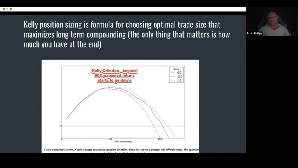
Why the curve peaks and declines: Large drawdowns take exponentially longer to recover from. A 50% drawdown requires a 100% gain to break even. A 75% drawdown requires a 300% gain.
Kelly optimal for Finrev: Based on historical 1.81 Sharpe performance, full Kelly is ~57% volatility target.
Conservative Kelly: Assuming 1.5 Sharpe forward (more realistic), optimal is ~50% volatility target.
Why You Should Trade BELOW Optimal Kelly
The formula assumes:
- Future performance matches past performance (unlikely to be exactly true)
- You have infinite emotional resilience (you don’t)
- You never panic-sell during drawdowns (you might)
Reasons to trade below optimal:
- Shorter time horizon: If you need returns within 3-5 years, you can’t afford multi-year drawdowns
- Psychological reality: Large drawdowns hurt worse than math suggests
- Conservative estimate: If you think the system might perform slightly worse than historical
- Portfolio context: If this is a large portion of your net worth
When to Trade ABOVE Optimal Kelly:
- Long time horizon (10+ years): Time smooths variance
- Small portfolio allocation: If this is <20% of net worth
- High stable income: Can add capital during drawdowns
- Exceptional conviction: Believe the system will outperform historical norms
- Youth: Decades to recover from mistakes
The personal choice: The founder of Finrev runs 50% volatility target (right at optimal Kelly with conservative assumptions). He’s been building trading systems for 20 years and has experienced 60%+ drawdowns before. He knows what he can handle.
Your choice: Should likely be 10-20% below whatever you think you can handle. Real drawdowns hurt worse than imagined ones.
Volatility Target Simulations: What to Actually Expect
Let’s run Monte Carlo simulations showing 10 random outcome paths for different volatility targets. This is what actually happens versus what backtests promise.
Setup: 1.5 Sharpe ratio system (conservative forward estimate), 3-year timeline, $10,000 starting capital
11% Volatility Target (Ultra-Conservative)
- Average annual return: 16%
- Best case: 23% annually
- Worst case: 11.3% annually
- Average max drawdown: 8.2%
- Longest drawdown: 268 days
- Ending capital range: $17,000 – $27,000
What this feels like: Boring. Steady. Occasionally frustrating when nothing happens. But even the unlucky outcome (bottom 10%) still makes money.
25% Volatility Target (Minimum for Most Users)
- Average annual return: 36%
- Best case: 58.5% annually
- Worst case: 13.2% annually
- Average max drawdown: 28%
- Longest drawdown: ~12 months
- Ending capital range: $19,000 – $38,000
What this feels like: Alternating between excitement and concern. Long flat periods punctuated by sharp moves up.
35% Volatility Target (Recommended Standard)
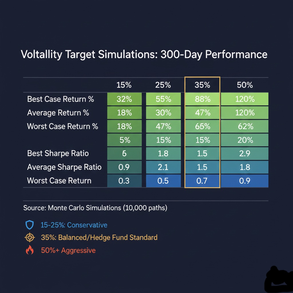
- Average annual return: 57%
- Best case (top 10%): 124% annually with only 18.9% max drawdown (dream scenario)
- Average case: 57% annually with 47% drawdown lasting 324 days
- Worst case (bottom 10%): ~30% annually with 53% drawdown lasting 470 days
- Average Sharpe ratio: 1.6
- Ending capital range: $25,000 – $95,000+
What this feels like: Occasionally magical, frequently frustrating, sometimes painful. You’ll question the system during 6-8 month flat periods. Then it’ll spike 40% in two months and you’ll feel brilliant.
The honest reality: Even the “worst case” here—30% annually with 53% drawdown—is objectively excellent. But living through a 470-day drawdown tests your conviction in ways spreadsheets can’t predict.
50% Volatility Target (Aggressive/Optimal)
- Average annual return: ~65%
- Best case: 164% annually with 37% drawdown
- Worst case: 31.6% annually with 61% drawdown lasting 488 days
- Ending capital range: $32,000 – $170,000+
What this feels like: Wild swings. Periods where you’re convinced it’s broken. Periods where you feel like a genius. Requires strong emotional control.
60% Volatility Target (Degenerate/Beyond Optimal)
- Average annual return: ~90%
- Best case: 300% annually (yes, really)
- Worst case: -5.8% annually (you lose money)
- Expected max drawdown: 60%
- Expected drawdown duration: 500+ days
Critical threshold: This is the first volatility level where losses appear in simulations. Out of 70 simulations run across all volatility targets, zero showed losses until reaching 60%.
Positive Skew vs. Negative Skew: Why It Feels Terrible to Win
Here’s a concept that determines whether you sleep well or constantly check your phone at 3 AM:
Skew: The shape of your return distribution
Negative Skew Systems (Most Retail Bots)

- Return pattern: Consistent small wins → Rare catastrophic losses
- Example: Win $100 on 65% of trades, Lose $1,500 on 35% of trades
- Feels like: Amazing! High win rate, steady profits, you feel smart
- Backtests like: Smooth upward curve, looks fantastic
- Reality: You’re selling insurance. You collect premiums (small wins) until the disaster strikes (large loss). The large losses don’t show up in backtests properly because they’re rare—but they’re inevitable.
Real-world example: FTX perpetual futures carry trade. Made money consistently… made money consistently… lost everything when the exchange collapsed.
Positive Skew Systems (Trend Following)
- Return pattern: Frequent small losses → Rare massive gains
- Example: Lose $50 on 60% of trades, Win $2,000 on 40% of trades
- Feels like: Terrible! Constant small cuts, feels like death by 1,000 paper cuts
- Backtests like: Flat… flat… flat… SPIKE… flat… flat… SPIKE
- Reality: You’re buying lottery tickets with positive expected value. Most tickets lose. But the winners are so large they more than compensate.
Why Positive Skew Allows Higher Leverage:
Positive skew systems can be traded at higher volatility targets without risk of ruin because they don’t blow up—they just go nowhere for a while.
The Honest Sales Pitch:
Most bots sell you: “70% win rate! Consistent daily profits!” (Translation: Negative skew system. You’ll love it until it blows up.)
What trend following actually is: “40% win rate. You’ll go months without profits. Then you’ll double your money in six weeks. Repeat.” (Translation: Positive skew system. You’ll hate it until you love it.)
Which would you rather:
- Feel smart consistently, then lose everything once?
- Feel dumb frequently, then get rich eventually?
Professional traders choose the second option. Retail traders choose the first, which is why retail traders lose, and professionals win.
Negative Skew (most retail bots):
- Pattern: Frequent small wins → Rare catastrophic losses
- Example: Selling insurance, carry trades, high win-rate strategies
- Feels: Amazing until it doesn’t (FTX perpetual carry trade scenario)
Positive Skew (trend following):
- Pattern: Frequent small losses → Rare massive gains
- Example: Buying lottery tickets with positive expected value
- Feels: Terrible until it’s amazing (months flat, then double your money)
Why it matters: Positive skew systems can handle higher volatility without blowing up. Negative skew systems feel good but eventually destroy capital.
The choice: Feel smart consistently then lose everything? Or feel dumb frequently then get rich eventually?
Choosing Your Volatility Target: The Framework
The optimal volatility target is the one you can live with without panic-selling. Here’s how to decide:
Start With These Questions:
1. Time Horizon
- <3 years: 25% volatility maximum
- 3-5 years: 35% volatility
- 5-10 years: 50% volatility
- 10+ years: Up to 60% volatility
2. Portfolio Allocation
- 50% of net worth: 25% volatility maximum
- 20-50% of net worth: 35% volatility
- <20% of net worth: 50% volatility
3. Income Stability
- Unstable: Reduce by 10-15 percentage points
- Stable: No adjustment
4. Drawdown Experience
- Never experienced 30%+ drawdown: Reduce by 10-15 percentage points
- Experienced and held through 50%+ drawdown: Can increase by 10 percentage points
| Volatility Target | Annual Return | Max Drawdown | Best For |
|---|---|---|---|
| 25% (Conservative) | ~35% | 33% for 283 days | <3 year horizon, 50%+ of net worth |
| 35% (Moderate) | ~50% | 43% for 382 days | 3-5 year horizon, 20-50% of net worth |
| 50% (Aggressive) | ~65% | 61% for 488 days | 5-10 year horizon, <20% of net worth |
| 60% (Degenerate) | ~90% | 60%+ for 500+ days | 10+ years, can tolerate losses |
Key insight: Whatever you calculate, reduce by 10-15%. Real drawdowns hurt worse than imagined ones.
First appearance of losses: 60% volatility target – below this, zero simulations showed losses over full backtest period.
Final recommendation: whatever you calculate, reduce by 10-15%. Real drawdowns hurt worse than imagined ones.
What HyperTrend Changes (And Doesn’t Change)
What DOESN’T change with the Hyperliquid vault migration:
- The underlying mathematics (Sharpe ratios, Kelly optimal, volatility targets)
- Expected return ranges for each volatility target
- Drawdown realities (trend following will always have long flat periods)
- Timeline requirements (still need 12-15 months minimum to judge)
What DOES change:
- Execution efficiency: 15-20% cost reduction through pooled capital fee advantages
- Position coordination: No more random execution queue luck across 2,000 accounts
- Faster signal access: Semi-HFT infrastructure enables previously untradeable signals
- Compounding enhancement: Small efficiency gains compound dramatically over years
The practical meaning: Same 1.5 Sharpe ratio expectations. But if Finrev delivered 50% annually at 35% volatility, HyperTrend might deliver 55-58% annually at the same volatility due to execution improvements.
Over 3 years: The difference is noticeable
Over 10 years: The difference is dramatic
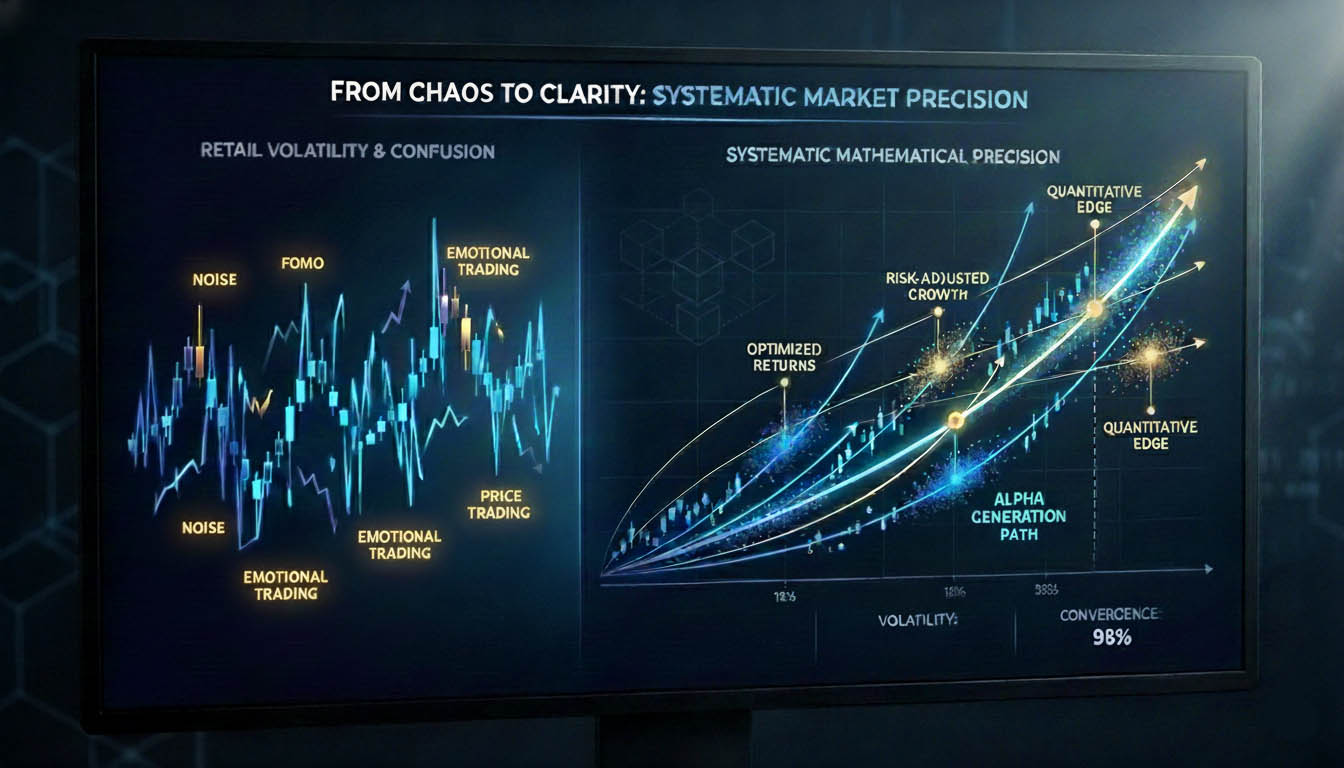
The Bottom Line: What Separates Winners from Losers
It’s not intelligence. Smart people lose constantly. It’s not capital. It’s not access.
It’s mathematics + psychology.
The mathematics:
- Measure performance by risk-adjusted returns (Sharpe ratio), not absolute returns
- Optimize position sizing through Kelly Criterion, not gut feel
- Blend uncorrelated signals for higher Sharpe ratios
- Trade positive skew strategies for psychological sustainability
The psychology:
- Choose volatility targets you can actually live with, not maximize
- Accept that 40% win rates can be more profitable than 70% win rates
- Understand that month 11 of a flat period might precede month 12’s breakthrough
- Resist the urge to abandon systems after 50-100 days of poor performance
The hedge fund advantage: They systematize the mathematics and remove the psychology.
Your advantage: You now understand the mathematics. Whether you can manage the psychology determines if you join the winners.
What DOESN’T change:
- The mathematics (still need 12-15 months to judge)
- Drawdown reality (trend following = long flat periods)
- Sharpe ratio targets (still 1.5+)
- Positive skew feel (will still be psychologically challenging)
What DOES change:
- 15-20% execution cost reduction (pooled capital advantages)
- Better position coordination (no random queue luck)
- Semi-HFT signal access (previously untradeable)
- Long-term compounding (small gains compound dramatically)
The honest pitch: Same Sharpe ratio. But 50% annual returns become 55-58% through execution efficiency. Over 3 years: noticeable. Over 10 years: dramatic.
Next Steps
If you want to go deeper:
- Why HyperTrend Is Rebuilding on Hyperliquid: The Infrastructure Evolution – Understand how execution improvements compound these mathematical advantages
- Inside the Finrev Team: Traditional Finance Meets Crypto Innovation – Meet the people applying this mathematics to real capital
If you’re evaluating Finrev/HyperTrend:
✅ Click here to watch the special introduction video with Scott to learn more about HyperTrend, Finrev, and the process of becoming a member.
✅ Once you have watched the “Introduction video,” you will be invited to book a call to talk to one of the onboarding coaches who are all actual traders.
✅ Understand this is a 5-10 year wealth-building journey, not a get-rich-quick scheme.
If you’re sceptical:
Good. You should be. Verify Scott’s vesting schedule on-chain when Trend coin launches. Track his personal wallets (he’s asking you to). Judge by actions, not words.
📄 Full Podcast Transcript: How Quants Engineer Forty Per cent Returns
Disclosure: This article discusses Finrev and HyperTrend systems. The author may have positions in the mentioned assets. This is educational content, not financial advice. Crypto trading involves substantial risk of loss. Past performance doesn’t guarantee future results. Sharpe ratios can vary significantly based on market conditions and timeframes. Monte Carlo simulations are probabilistic models, not guarantees. Do your own research before investing.